What Is the Vacuum? From Empty Space to a Structured Medium

Ask most people what is left when you remove every atom from a box, and they say: nothing. Empty space. Zero.

Before the argument, the picture. Below are the two ways people draw the lowest state of the simplest quantum system there is — a mass on a spring, cooled as far as cooling goes. One is a bead on a trajectory, rattling too fast to see. The other is what the mathematics says: a spread over position that does not change with time at all. Under each picture is a clock, and only one of them has anything to count.

A stationary spread, not a fast jitter

Two pictures of the same ground state, side by side. Switch between them and watch the clocks. One picture has a bead swinging in a bowl and a clock counting periods; it is the intuition most readers arrive with, and this chapter teaches against it. The other is the state as it actually is — a spread over position that holds half a quantum and does not change with time at all. Its clock is greyed out because there is nothing for it to count.

Which picture are you looking at?

Show me the trajectory pictureShow me the state

Show me the trajectory picture

The picture this chapter is teaching against

Here is the bead in the bowl. It has a position at every instant, it swings out to a turning point and back, and a clock underneath it counts the periods. This is a fair intuition for one thing only: an energy you cannot remove, because nothing you do brings this bead to rest. It is worth looking at carefully, and it is worth knowing what it is not: there is no hidden classical path underneath the quantum ground state for this bead to be tracing.

Clock: 0.00 periods

Show me the state

Nothing here changes with time, so this clock is stopped.

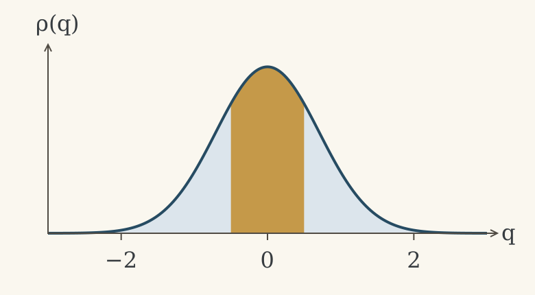
Here is the state. The spread over position is the whole of it — measure many independently prepared oscillators and this is how the results are distributed. Nothing in this panel changes with time, so the clock beneath it has nothing to count. The uncertainty principle forbids a definite position together with a definite momentum; it does not hide a trajectory under a blur. The spread is the state.

Clock: —

The clock runs only under the trajectory picture, because only the trajectory picture has anything that changes.

Run the clockBack to the start

Time on the clock

0.00

Ground-state energy

half a quantum, ½ħω

Share of measurements landing inside the shaded band

52%

OpenStax, University Physics volume 3, §7.5, the quantum harmonic oscillator — the stationary ground state and ½ħω, as taught

The state: a stationary spread over position holding half a quantum. The clock is stopped because nothing in this panel changes with time. Nothing here changes with time, so this clock is stopped.

Modern physics says the opposite, and this is not a fringe opinion. It is the mainstream, textbook core of the field. Empty space is the lowest state of every field in nature, and that state is not nothing. The rest of this book is about taking that sentence completely seriously.

The aether never really died — it changed clothes

For centuries physicists believed in the aether: an invisible mechanical medium that light waves rippled through, the way sound ripples through air. In 1887 the famous Michelson–Morley experiment failed to detect motion through it. Einstein's relativity then made the mechanical aether unnecessary. Case closed — or so the textbook story goes.

What happened next is more interesting than that story, and it is worth stating exactly, because the sloppy version hands a critic a free win. Quantum field theory does not restore that mechanical model. It says something different, and in the end stranger:

• Quantum theory says a vacuum is a state of the fields, specified for a physical system: the lowest-energy one. It is not a substance poured into a container. What makes it remarkable is that the lowest state is not "off" — measure a field in it and the results still have a spread that no cooling, damping or shielding removes.
• General relativity says spacetime carries a metric: the rule that fixes the interval between events, and with it the bending we call gravity. The metric is not a sheet with weights resting on it, and it is not a fluid draining inward. Those are drawings of the mathematics, not the thing.

Nobel laureate Frank Wilczek put the modern view plainly in The Lightness of Being. Is space an empty stage, or "the primary reality of which matter is a secondary manifestation"? His answer: "Today the third view is triumphant." The vacuum is the main character.

Zero-point energy: the spread that never goes away

Here is the first piece of hard physics. Solve a quantum oscillator — a mass on a spring, a molecule stretching, one note on a string — and you get a ladder of allowed energies. The bottom rung is not zero. It sits half a step up, measured from the minimum of its potential.

Ground-state energy of a harmonic oscillator(2.1)

$$E_0 = \tfrac{1}{2}\hbar\omega$$

This is zero-point energy (ZPE), and it is not speculative. It is why liquid helium refuses to freeze solid under its own vapour pressure, and it shows up throughout chemistry and spectroscopy. In later chapters the live question is never whether zero-point energy exists. It does. The question is how far it can be shaped, tapped, or engineered.

One picture trips readers constantly, so fix it here. The ground state is not a bead rattling in a bowl too fast to see. Its probability distribution is stationary — it does not change with time at all. What the uncertainty principle forbids is a state with both a definite position and a definite momentum; it does not smuggle a hidden classical trajectory in underneath. The spread is the state, not a blur over motion. The standard undergraduate treatment is worth reading directly: OpenStax, University Physics Volume 3, §7.5.

The two panels at the top of this chapter are that distinction drawn, and they are worth going back to now that the ½ħω is on the page. What they put in the foreground is a probability density over position — measure many independently prepared oscillators and about 52% of the results land within half an oscillator length of centre, with tails running past both edges of the view.

One more piece of vocabulary. The zero in zero-point energy means one thing only: zero thermal temperature. Douglas Miller, who is building a chip to tap the field, states it as flatly as it can be stated: "You take all thermal energy out, now you're absolute zero temperature. That's the zero part of zero point energy. It should not be confused in any other way." It is the floor of the thermal scale, not the floor of energy.

The zero is a thermometer reading

The name misleads almost everybody who meets it. Run the temperature of one mode of the field down towards absolute zero and watch what happens to the two things it carries: the thermal part drains away to nothing, and the half-quantum underneath it does not move at all. That half-quantum is what is left at the zero of the thermal scale, which is the only zero the name is about. Set the temperature and the mode, and read both parts off separately.

The mode, and how warm it is

Temperature

300 kelvin

Wavelength of the mode you are watching

1 mm

• Where a gold mirror stops reflecting: 136 nm
• The infrared field the sampler on this page reads directly: 1.18 µm

Back to the opening setting

• The zero-point floor — half a quantum, at every temperature
• The thermal part — all of what a thermometer reads
• Where the two are exactly equal

Zero-point floor:

0.5 quanta

Thermal part:

20.4 quanta

Mean energy of the mode:

20.9 quanta

Share of the energy that is thermal:

97.6%

Frequency of that mode:

300 GHz

Temperature at which the thermal part equals the floor:

13.1 kelvin

What this shows: This mode is warm enough that most of what it carries is thermal, and a thermometer would read nearly all of it. Notice what has not happened: the floor underneath is exactly the same half-quantum it was at the coldest setting. It became a smaller share of a larger total, which is a different statement from going away.

So the sentence to write is that the zero in zero-point energy means zero thermal temperature, and nothing else. It is the floor of the thermal scale, not the floor of energy, and a reader who takes the name to mean nothing is there has been handed the wrong picture by the word.

Scope: one mode of a field in thermal equilibrium, drawn from the Planck mean occupancy — the standard textbook accounting, and not a model of any apparatus. The three constants it runs on are defined values of the international system of units, exact rather than measured.

The sheets this wording answers to

• Douglas Miller states the correction on air: the zero refers to thermal temperature and nothing else
• Observation of the thermal Casimir force — the laboratory case where the thermal part is the larger of the two

Now the step that turns an oscillator into a field. Quantise the electromagnetic field and every mode — every wavelength, direction and polarisation — behaves like one of these oscillators, each keeping its own ½ħω. There is no shortest wavelength in the idealised problem, so the unrestricted sum diverges: it is a formal expression, not a measured quantity. What laboratories measure are differences in this energy when boundaries or materials change. That distinction is the whole reason the next section is an experiment instead of an argument.

That half-quantum in every mode is not only an entry in an inventory. It is a field that does work on matter, and the oldest test case is the simplest atom. A classical electron circling a proton accelerates, an accelerating charge radiates, and the Bohr atom should therefore drain itself into the nucleus in about ten picoseconds. Hal Puthoff's 1987 paper writes down the other side of that ledger: the orbiting electron is also absorbing power from the zero-point field it is immersed in. Set the two rates equal and the ground state stops being a postulate and becomes a balance point — and the radius at which the balance sits comes out as exactly the Bohr radius, with nothing fitted. Move the radius yourself and watch which rate wins.

Why the hydrogen atom does not collapse

In the classical picture an orbiting electron radiates, so the atom should spiral in and collapse. Puthoff's 1987 result is a balance: the power the orbiting electron radiates away equals the power it absorbs from the zero-point field of the vacuum, and the orbit radius at which those two rates are equal comes out at the Bohr radius. Move the radius and watch which rate wins.

Orbit radius

Orbit radius, in Bohr radii

0.73

Return to the Bohr radius

• Power radiated away
• Power absorbed from the zero-point field

What is happening: Inside the balance point the electron absorbs more from the vacuum than it radiates away, so the orbit is pushed back out.

Absorbed divided by radiated: 1.17

Scope: this is a stochastic-electrodynamics result at the level of the Bohr theory. It defines the ground state as a balance and answers radiative collapse; it does not replace quantum mechanics and does not derive the full hydrogen spectrum.

The source sheet: Puthoff 1987, Ground state of hydrogen as a zero-point-fluctuation-determined state

How far the idea has been taken

The balance above is the first rung of a ladder researchers have been climbing ever since. Each rung asks more of the same idea.

1. 1987 — Puthoff builds the circular orbit from two one-dimensional oscillators a quarter cycle apart, and the balance closes at the Bohr radius.
2. 2003 — Cole and Zou put a classical electron and a classical zero-point field on a computer; the time it spends at each distance converges on the quantum ground-state curve.
3. 2015 — Nieuwenhuizen and Liska run the full three-dimensional atom for far longer; short runs trend toward the quantum result, and long runs ionise.
4. 2016 — Nieuwenhuizen locates the threshold: stretched orbits with angular momentum below 0.588 in units of the reduced Planck constant gain energy every revolution, and an added repulsive term is predicted to hold them.
5. A second road — Nelson's 1966 stochastic mechanics gives every particle a frictionless random motion and recovers the Schrödinger equation, with the ground state as a dynamical equilibrium and no electromagnetic zero-point field invoked.

What would settle it: A three-dimensional stochastic-electrodynamics atom that holds its ground state over long runs, with the origin of any added term identified — or a measured difference between the field picture and the purely stochastic one.

That result is a stochastic-electrodynamics calculation at the level of Bohr theory: a classical particle, a classical field and a circular orbit. It does not replace quantum mechanics and it does not derive the full hydrogen spectrum, and the paper states that scope itself. The abstract, the located claims and a full walkthrough of the balance argument are on the source sheet: Puthoff 1987, the ground state of hydrogen as a zero-point-fluctuation-determined state.

Puthoff's balance is an argument about the field; there is also a measurement of it. A probe pulse far shorter than one cycle of the infrared vacuum field can sit on that field and read its amplitude directly. Stretch the probe below, or widen the spot, and the reading falls — exactly as averaging over more of the field says it must.

Reading the vacuum's own field

A laser pulse lasting less than one and a half cycles of its own light crosses a crystal, and whatever electric field is present at that instant twists its polarisation. Made short enough, the pulse resolves the infrared vacuum inside a single cycle, and the vacuum's own fluctuations appear as extra noise riding on the laser's. Eighteen volts per centimetre, against a prediction of twenty point two, with no amplifier anywhere in the chain.

What the instrument reads

Where in the cycle the probe lands

0.0

Probe pulse duration

5.8

Spot radius at the crystal

4.25

Probe photons per pulse

1E8

Sweep the probe across the cycleReturn to the published settings

• The infrared vacuum field
• The probe pulse
• Predicted from mode counting

Vacuum field amplitude at this sampling volume:

18.0 volts per centimetre

Predicted from mode counting:

20.2 volts per centimetre (89.11%)

Sampled four-volume, against the published one:

1E0×

Cycles of its own light the probe lasts:

1.48

Excess in normalised noise amplitude:

4.7%

Field the probe actually resolves, as a share of the full amplitude:

57.95%

What the instrument reads: 18.0 volts per centimetre. 4.7%. Inside the usable window. The measurement disturbs the field it is listening to only at third order, which at these intensities is negligible — effectively back-action free.

Eighteen volts per centimetre read against twenty point two predicted. The agreement is the reason the reading is trusted, and the two controls are the reason it is the vacuum rather than the instrument.

There is an upper limit to how hard the probe may be pushed, worked out separately: below the window shot noise buries the signal, and above roughly a hundred billion photons per pulse the probe begins to create the photons it is measuring. The published experiments run near a hundred million, comfortably inside. (1.6E11)

Inside the usable window. The measurement disturbs the field it is listening to only at third order, which at these intensities is negligible — effectively back-action free.

• The source sheet: direct sampling of electric-field vacuum fluctuations
• The back-action window the reading has to stay inside
• Separating the vacuum's own fluctuations from a source's radiation

Measuring the Casimir interaction

In 1948 the Dutch physicist Hendrik Casimir worked out a difference you can put on a bench. Place two uncharged, perfectly conducting plates very close together in vacuum, and the modes that fit between them are not the modes that fit outside. Change the separation and that energy changes. An energy that changes with distance is a force.

Casimir pressure between ideal plates(2.2)

$$\dfrac{F}{A} = -\dfrac{\pi^2 \hbar c}{240\, a^4}$$

A number you can check. With a gap of 1 µm, equation 2.2 gives about 1.3 millipascals. Over a plate area of one square centimetre that is about 0.13 micronewtons — small, and well inside what a torsion balance can feel. Both figures are the ideal model, not the reading of any instrument.

Lamoreaux, 1997. Steve Lamoreaux hung a torsion pendulum in a vacuum chamber and brought a flat plate toward a spherical lens over separations from 0.6 to 6 micrometres. He reported agreement with theory at about the 5% level, and the publisher lists a 1998 erratum that belongs with the paper. Forty-nine years after the prediction, the vacuum's push had a number on it. A year later a second group used a different instrument — Mohideen and Roy's atomic force microscope — and reached about the one-percent level. Independent instruments in independent laboratories agreeing is what turns a result into a fact.

Read carefully what those measurements establish, and what they do not. They establish that the electromagnetic ground state couples to matter and exerts a calculable force whose sign can be engineered. They do not hand you the absolute energy density of empty space. Robert Jaffe's 2005 paper is the sharpest statement of the distinction: the same force follows from the fluctuating charges and currents in the plates, with no zero-point reservoir appearing in the bookkeeping at all. The force is real either way, and the coupling to matter is where any energy ledger has to be written.

Closing the gap does not empty it, either. The plates shut out the longest waves, the few carrying the least energy; everything shorter and more energetic stays exactly where it was. Miller puts a number on it: "basically the entire 99.99% of the force of the zero point energy is still inside." So negative energy between plates is a naming convention, not an exotic substance. Say below the ambient vacuum level, never below nothing. That also flips the engineering problem: you are not emptying a box, you are standing on the shore of an ocean asking how to reach deeper. The derivation, the real-material corrections and the device programmes have their own course: the zero-point field and the Casimir effect.

Count that sliver yourself. Set the gap, choose how short a wave the field still couples to, and the ladder of modes that fit redraws — with the share of the zero-point energy the closing plates actually exclude stated as a number beside it.

Count the modes the gap shuts out

A wave only fits between two plates if a whole number of half-wavelengths spans the gap, so the longest wave the gap can hold is twice the separation. Closing the plates shuts out the waves longer than that — the few carrying the least energy — and everything shorter stays exactly where it was. Move the separation and watch the ladder of allowed modes redraw, and watch what share of the zero-point energy in that volume the closing gap actually excludes.

Plate separation

Separation between the plates

1,000

Return to one micrometre

Shortest wavelength the field still couples to

About 136 nanometres — a gold mirror stops reflecting above its plasma frequency10 nanometres — extreme ultraviolet1 nanometre — soft X-ray

• Modes that fit in the gap
• Too long to fit — what the gap shuts out

Modes that fit, up to the cutoff:

14

Longest wave the gap holds:

2,000 nm

Share of the zero-point energy in that volume the gap excludes:

0.077%

Share still inside the gap:

99.9229%

What this shows: The excluded sliver is thin. Almost all of the zero-point energy in that volume is still inside the gap, and the measured force comes from the thin excluded sliver alone. This is why negative energy between plates is a naming convention rather than a substance: say below the ambient vacuum level, never below nothing.

About 136 nanometres — a gold mirror stops reflecting above its plasma frequency

Scope: a one-dimensional scalar field with a sharp shortest wavelength — the standard teaching model for mode counting and the energy bookkeeping. It is not a computation of any laboratory force, and it asserts no absolute energy density of empty space. The force laws and the real-material corrections belong to Lifshitz and scattering theory.

Where this is worked through: the zero-point field and the Casimir effect

"Vacuum engineering" is a phrase a Nobelist coined

The step from "the vacuum has structure" to "maybe we can alter it" is not something we invented. Nobel laureate T. D. Lee wrote it into his standard textbook: "The experimental method to alter the properties of the vacuum may be called vacuum engineering… If indeed we are able to alter the vacuum, then we may encounter new phenomena, totally unexpected."

That single sentence is the seed of this entire field. A declassified U.S. Defense Intelligence document (Chapter 4) opens by quoting exactly this line. It then proposes that "empty space itself might be engineered to provide energy/thrust." How far that proposal can be carried is what the rest of this book grades, one rung at a time.

The vacuum has irreducible zero-point energy and exerts measurable forces; spacetime has a metric structure. The device research in later chapters asks how these properties could supply useful energy or propulsion, and how to measure the complete energy and momentum exchanges.

Energy accounting over a full cycle

The standard objection to everything downstream deserves to be met head-on, because the answer is arithmetic rather than opinion. The vacuum is the ground state, and you cannot draw work from the lowest energy level.

Take the clean case first. For a fixed attractive force with the materials held constant, letting two plates come together releases energy and pulling them apart costs exactly that energy back. In the reversible limit the two are equal; any real friction or dissipation only adds to the bill. A device that returns to its exact starting condition and claims net work out has not found a loophole in that arithmetic.

But "the device came back to its starting state" is not the same as "the books balance", and this is where arguments on both sides go wrong. The device is not the whole system. An external source may have supplied work along the way — changing a material, driving a field, moving a boundary. So the ledger a result has to close is the complete one: the external energy inputs, the changes in stored energy, and the output actually delivered to a load, with calibration and uncertainty attached. Cole and Puthoff's 1993 analysis concluded that the proposals it examined are correct in principle, and it explicitly left technological implementation outside its scope. A real result and a real limit, in one sentence.

Draw the boundary before you count

A windmill turns for as long as the wind blows, and nobody calls it a perpetual-motion machine. The reason is the whole lesson: the wind is drawn inside the ledger. The second law of thermodynamics says the entropy of an isolated system does not fall. A windmill, a sailboat and a drill biting steadily into wood are not isolated. Energy crosses their boundary all the time, and an open system held away from equilibrium by that flow can do steady work for as long as the flow lasts, without breaking the first law or the second. Tom Bearden taught the point with exactly these examples, and Ashton Forbes replayed that lesson on his 12 September 2026 stream.

That is the frame every vacuum-coupled device has to be measured in. The thesis is that the zero-point field is an environment of this kind — a wind that never stops. So the engineering question is never "does it violate conservation?" It is: where is the boundary drawn, what crosses it, and has every crossing been measured? Name the inflow, account for every store of energy inside, and measure what reaches the load.

A switched-coil motor, read as an engineering card

Yoshiaki Takahashi's United States patent 5,861,693 (1999) is a buildable example of the kind of machine this ledger is written for. It is a brushless motor: a Hall-effect sensor sees a rotor pole arrive, switches on the next stator coil so its core pulls the pole forward, and the previous coil's current dies away as the pole leaves. Each rotor pole carries a very strong two-layer permanent magnet, and beside every drive coil sits a second coil that generates power as the poles sweep past, tuned by a capacitor for low speed. Its stated aim is long running from a starting input while storing power. The patent describes the architecture; the test requires real power in and real power out over a long, closed run with every battery and capacitor accounted for.

The first step of that measurement is the one most often skipped. Try it below.

Measure a motor properly

A voltmeter reading times an ammeter reading is not the power a machine takes. Shift the current out of step, add distortion, change the meter, and compare what the meters multiply to the power that does work.

The load and the meters

How far the current lags the voltage

0 degrees

Distortion in the current (third harmonic)

0% of the fundamental

Ammeter typeTrue-RMS meterAverage-responding meter, scaled for a sine

Clean, in-step load

• Voltage
• Current
• Meter volts × meter amps
• Real power

What the numbers say: Current in step and undistorted: the meter product and the real power agree. Only in this case is volts times amps the power.

Meter volts × meter amps:

1.00 per unit

Real power:

1.00 per unit

Power factor:

1.00

Meter product divided by real power:

1.00

What turns a demonstration into evidence

1. Measure real power on both sides with an instrument that multiplies voltage and current at every instant, not two separate meters.
2. Use the same kind of instrument, calibrated, on the input and the output.
3. Record the charge of every battery and capacitor at the start and the end, and run long enough that their change is small against the output.
4. Close the loop where possible, so the machine runs from its own output with the external supply disconnected.
5. Publish the waveforms, the instruments and the raw log, so another bench can repeat it.

Scope: a sinusoidal voltage with a current that lags and carries one harmonic. Real machines can distort the voltage too and draw several harmonics; the principle, average the instantaneous product, is the same.

A machine this standard applies to: Takahashi's switched-coil generating motor patent

That is why the route the field is actually taking is not "cycle the ground state for free". It is: shape the vacuum's own spectrum with a cavity, then measure what that does to matter. The complete accounting, the funded device programmes and the measurement that would settle them are worked through in the zero-point field and the Casimir effect, and Chapter 6 takes up the energy question directly.

The strongest objection, answered

The objection · Standard thermodynamics

“The vacuum energy is real, but it is the ground state — and you cannot draw work from the lowest energy level.”

The answer

Agreed, for the case that arithmetic covers: a closed cycle at fixed materials returns exactly what it released, and no arrangement of plates escapes that. The physics underneath is worth knowing exactly, too. Robert Jaffe showed in 2005 that the Casimir force follows from ordinary quantum electrodynamics — the fluctuating currents in the plates themselves — without invoking zero-point energy at all, and it fades as the fine-structure constant goes to zero. So the Casimir measurement proves the vacuum couples to matter and exerts a real force; on its own it does not hand you a supply to draw from.

What the objection does not settle is the open, driven, asymmetric case, where an external source is part of the ledger and the question is whether anything useful can be rectified out of it. That is an engineering question with a stated bar in front of it, not a thermodynamic contradiction, and Chapter 6 works through which schemes clear the accounting, which do not, and what to watch next.

What the field added — July to September 2026

Two distinct 2026 papers report cavity-enhanced superconductivity in NbSe₂, and keeping them apart matters. Wang and colleagues, in Nature, placed a thin flake inside a terahertz "dark cavity" that reshapes vacuum fluctuations with no drive field, and report a rise in the superconducting transition temperature along with the critical current and critical field. Separately, a preprint by Zhang and colleagues (arXiv:2606.19171v2) reports a bilayer moving from 3.02 K to 3.41 K in a 0.92 THz resonator. Two groups, two apparatus, two author lists — not two versions of one paper. Both report changes in a material's superconducting properties; they are not measurements of energy delivered by a cavity to a load.

The Wang paper describes a material measurement, with independent replication still needed. The Casimir force showed that the vacuum pushes on plates. These results say something new: reshape the vacuum's spectrum around a material and the material's own quantum state changes. That is the mechanism the device chapters are built on, and it is now in the peer-reviewed literature.

The season also revisited the aether with modern tools, and the history is easier to check than the anecdotes about it. Dirac published a letter titled "Is there an Æther?" in Nature in 1951, arguing that his own reformulation of electrodynamics pointed back toward a preferred state of space. Puthoff's 1987 paper in Physical Review D then modelled the hydrogen ground state as a balance between radiated and absorbed power in the zero-point field — a result obtained within stochastic electrodynamics at the level of Bohr theory, which is exactly how strong it is and exactly how far it reaches. The drill-down from a first picture to the device programmes is the course: the zero-point field and the Casimir effect.

What would settle the next step: an independent group reproducing the dark-cavity rise in transition temperature, in a different material and a different laboratory, with the cavity's own drive and losses accounted for. Precision Casimir measurements already match equation 2.2 to the percent level once real materials are folded in, which is why the rest of the book can stand on this chapter.

Sources

Theory and history

• H. B. G. Casimir (1948), "On the attraction between two perfectly conducting plates," Proc. K. Ned. Akad. Wet. 51, 793–795 — the prediction this chapter rests on; bibliographic record.
• H. B. G. Casimir & D. Polder (1948), "The Influence of Retardation on the London–van der Waals Forces," Phys. Rev. 73, 360; DOI 10.1103/PhysRev.73.360. /library/stm-e472d5f70d.
• P. A. M. Dirac (1951), "Is there an Æther?", Nature 168, 906–907 — the letter quoted above; publisher record.
• T. D. Lee, Particle Physics and Introduction to Field Theory (1981) — "vacuum engineering" is Lee's own term; book record.
• F. Wilczek, The Lightness of Being (Basic Books, 2008) — the mainstream anchor that a structured vacuum is orthodox quantum field theory; book site.
• OpenStax, University Physics Volume 3, §7.5, "The Quantum Harmonic Oscillator" — the stationary ground state and ½ħω, as taught; open textbook section.

Measurements

• S. K. Lamoreaux (1997), "Demonstration of the Casimir Force in the 0.6 to 6 µm Range," Phys. Rev. Lett. 78, 5 — torsion pendulum; agreement reported at about the 5% level; DOI 10.1103/PhysRevLett.78.5.
• S. K. Lamoreaux (1998), erratum to the 1997 measurement, Phys. Rev. Lett. 81, 5475; DOI 10.1103/PhysRevLett.81.5475.
• U. Mohideen & A. Roy (1998), "Precision Measurement of the Casimir Force from 0.1 to 0.9 µm," Phys. Rev. Lett. 81, 4549 — a different apparatus in a different laboratory; DOI 10.1103/PhysRevLett.81.4549.

Where the derivations are worked out

• R. L. Jaffe (2005), "Casimir effect and the quantum vacuum," Phys. Rev. D 72, 021301 — the same force derived from the plates' own fluctuating currents; arXiv:hep-th/0503158.
• K. Milton (1999), "The Casimir effect: physical manifestations of zero-point energy" — sign and geometry dependence, including Boyer's repulsive sphere; arXiv:hep-th/9901011.
• H. E. Puthoff (1987), "Ground state of hydrogen as a zero-point-fluctuation-determined state," Phys. Rev. D 35, 3266 — obtained within stochastic electrodynamics at the level of Bohr theory; DOI 10.1103/PhysRevD.35.3266.

Recent cavity reports

• Z. Wang, G. Cardoso, L. Yang et al. (2026), "Evidence for vacuum-enhanced superconductivity in NbSe₂," Nature, published 19 August 2026; DOI 10.1038/s41586-026-11037-x.
• H. Zhang, Z. Feng, I-T. Lu et al. (2026), "Cavity-enhanced superconductivity in the two-dimensional limit of NbSe₂," preprint, v2 revised 19 August 2026; arXiv:2606.19171v2.