Quantum mechanics I–II
Develop Hilbert-space states, operators, dynamics, spin, approximation methods, and identical particles.
Move from wave mechanics into the formal structure needed for quantum fields, vacuum states, Casimir physics, condensed matter, and critical reading of quantum-technology claims.
Interactive model
Explore before calculating
Live laboratory
Quantum bound-state spectrum
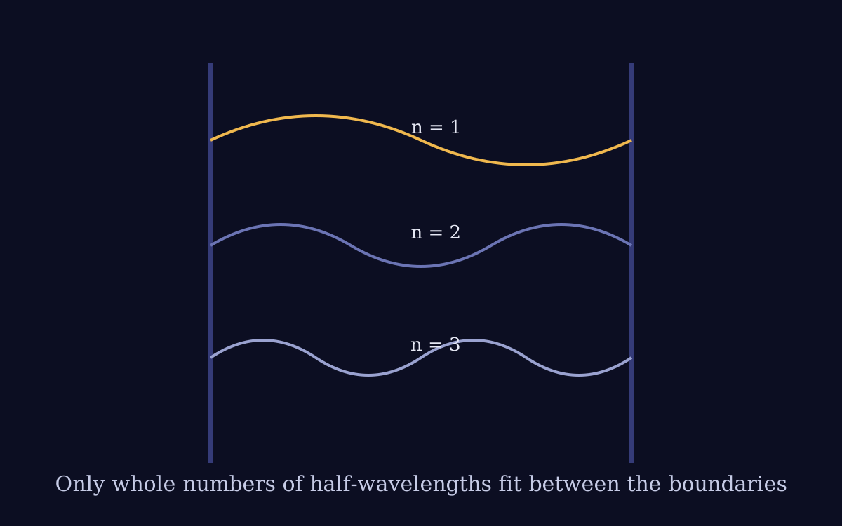
Change an infinite well and its particle mass. Boundary conditions select discrete energies whose spacing scales with n², inverse mass, and inverse width squared.
Ground energy: 0.376 eV
Selected energy: 0.376 eV
E1/E1: 1
Allowed n: 1, 2, 3, …
The missing n=0 is not a hidden zero-energy state: it would make the wavefunction identically zero under both boundaries and cannot represent a normalized particle.
Level 3 · Undergraduate core teaching kit
Record the investigation. Teach the reasoning.
A learner-facing lab record and a course-specific instructor guide turn the live model into a repeatable classroom investigation.
Learner record
Discrete spectrum and basis-state audit
How do Hamiltonian parameters and boundary conditions determine allowed energies and measurement probabilities?
Download learner recordInstructor guide
Teach for evidence, not button pushing
Learners connect a specified Hamiltonian and boundary conditions to a normalized discrete spectrum without universalizing one model.
Download instructor guideLesson 1 of 3
Hilbert space, states, and operators
How does linear algebra encode preparation, evolution, and measurement?
A pure state is a normalized vector up to global phase. Observables are Hermitian operators; eigenvalues are possible outcomes and projections set probabilities.
Noncommuting operators cannot share a complete sharp basis, producing structural uncertainty relations.
Worked example
For normalized |ψ⟩=(|0⟩+i|1⟩)/√2, find probabilities in the {|0⟩,|1⟩} basis.
- 1. Project onto |0⟩ and |1⟩.
- 2. Amplitudes are 1/√2 and i/√2.
- 3. Square magnitudes.
Each outcome has probability 1/2; relative phase matters in other bases.
Try it
Basis rotation
Materials: Notebook with two-component complex vectors.
- 1. Define computational and rotated bases.
- 2. Project one state into each.
- 3. Verify probability normalization.
- 4. Vary relative phase.
Notice: Probabilities depend on measurement basis while the state vector transforms consistently.
Check your understanding: Why must observable operators be Hermitian?
Answer: They have real eigenvalues and orthogonal spectral structure suitable for measurement outcomes.
Hermiticity supports real expectation values and unitary basis decomposition.
Lesson 2 of 3
Schrödinger dynamics and bound states
How do a Hamiltonian and boundary conditions determine allowed energies?
The time-dependent Schrödinger equation generates unitary evolution. Separating time for a time-independent Hamiltonian yields an eigenvalue problem.
Boundary conditions and normalizability quantize bound-state energies. Tunneling follows from nonzero wavefunction amplitude in classically forbidden regions.
Worked example
Find infinite-well energies for width L.
- 1. Inside, solve ψ″+k²ψ=0.
- 2. Enforce ψ(0)=ψ(L)=0.
- 3. Obtain k=nπ/L.
- 4. Use E=ℏ²k²/(2m).
Eₙ=n²π²ℏ²/(2mL²), n=1,2,…
Try it
Finite-well eigenvalue search
Materials: Numerical notebook.
- 1. Define a finite square well.
- 2. Integrate trial energies.
- 3. Detect boundary mismatch.
- 4. Root-find allowed energies and plot states.
Notice: Finite barriers shift energies and produce exponentially decaying tails.
Check your understanding: Why is n=0 absent in the infinite well?
Answer: It gives the zero wavefunction under both boundary conditions, which cannot be normalized as a physical state.
The first nontrivial standing mode is n=1.
Lesson 3 of 3
Spin, composites, and approximation methods
How do intrinsically quantum degrees of freedom and approximations extend solvable models?
Spin-1/2 states live in a two-dimensional complex space and transform under rotations differently from classical arrows. Composite systems use tensor products and can be entangled.
Perturbation theory and variational methods estimate systems near or above exactly solvable cases, with explicit convergence and trial-state limits.
Worked example
A spin-up-z state is measured along x. What probabilities result?
- 1. Write |↑z⟩=(|↑x⟩+|↓x⟩)/√2.
- 2. Project onto x eigenstates.
- 3. Square amplitudes.
Up-x and down-x each occur with probability 1/2.
Try it
Variational ground-state estimate
Materials: Notebook and a parameterized trial wavefunction.
- 1. Normalize the trial state.
- 2. Compute ⟨H⟩ versus parameter.
- 3. Minimize numerically.
- 4. Compare with a known benchmark.
Notice: The variational minimum is an upper bound to the true ground energy within the modeled Hamiltonian.
Check your understanding: Does entanglement allow controllable faster-than-light messaging?
Answer: No.
Local outcomes remain random; correlations require classical comparison and respect no-signaling.
Formula-to-meaning deck
Read the equation in ordinary language.
iℏ∂|ψ⟩/∂t=H|ψ⟩
The Hamiltonian generates unitary quantum-state evolution.
⟨A⟩=⟨ψ|A|ψ⟩
Expectation value averages observable outcomes in a state.
ΔAΔB≥½|⟨[A,B]⟩|
Noncommuting observables impose a state-dependent uncertainty bound.
Independent practice
Problem set
Work each problem before opening its hint and solution.
1. Normalize ψ(x)=Ae⁻ᵃˣ on x≥0 for a>0.
Reveal hint
Set ∫|ψ|²dx=1.
Reveal solution
A=√(2a), choosing positive real phase.
2. For [x,p]=iℏ, recover the position-momentum uncertainty bound.
Reveal hint
Use the general commutator inequality.
Reveal solution
ΔxΔp≥ℏ/2.
3. A perturbation λx shifts a parity-even ground state at first order by what amount?
Reveal hint
Evaluate λ⟨0|x|0⟩ and use parity.
Reveal solution
Zero first-order shift for an even state in a parity-symmetric unperturbed system.
Derivation studio
Build the result, line by line.
Keep the assumptions visible so the mathematics remains auditable.
Starting point
Infinite square-well spectrum
−(ℏ²/2m)ψ″=Eψ on 0<x<L
- 1. Set k²=2mE/ℏ².
- 2. Solve ψ=A sin kx+B cos kx.
- 3. Apply ψ(0)=0 to set B=0.
- 4. Apply ψ(L)=0 to require kL=nπ.
Eₙ=n²π²ℏ²/(2mL²)
Energy quantization comes from wave dynamics plus boundary conditions.
Starting point
First-order perturbation energy
H=H₀+λV and |n⟩ expansion in λ
- 1. Insert series into H|ψ⟩=E|ψ⟩.
- 2. Collect first-order terms.
- 3. Project with ⟨n⁰|.
- 4. Use orthonormality and H₀ eigenvalue relation.
Eₙ^(1)=⟨n⁰|V|n⁰⟩
First-order shift is the perturbation's expectation in the unperturbed state.
Computational notebook
Turn the model into an experiment.
Wave-packet evolution
How do dispersion and barrier scattering reshape a Gaussian packet?
Inputs
- • Packet center, width, mean momentum
- • Grid and time step
- • Free or barrier potential
Algorithm
- 1. Construct and normalize ψ.
- 2. Propagate with a stable split-step or Crank–Nicolson method.
- 3. Track norm and energy.
- 4. Measure reflection, transmission, and spreading.
Evidence to produce
- • Space-time probability-density plot
- • Norm/energy conservation diagnostics
- • Reflection and transmission versus energy
Continue into the evidence